
目录
在Python开发的实际工作中,特别是在Windows环境下进行数据分析和上位机开发时,我们经常面临这样的挑战:如何高效地从大型数组中提取特定数据?如何灵活地改变数据的形状以适应不同的计算需求?如何处理多维数据结构?
这些看似复杂的问题,实际上都指向了NumPy中三个核心概念:数组索引、切片操作和形状变换。很多Python初学者在这里容易卡壳,不是因为概念本身复杂,而是缺乏系统的实战指导。
本文将从实际应用场景出发,通过丰富的代码示例和Windows环境下的编程技巧,带你彻底掌握NumPy数组的索引、切片与形状操作。无论你是数据分析新手,还是正在从事科学计算、图像处理的工程师,这些技能都将成为你Python开发路上的重要基石。
🔍 问题分析:为什么这三大技能如此重要?
在深入学习之前,让我们先理解一个核心问题:为什么数组索引、切片和形状操作是NumPy编程的必备技能?
实际应用场景分析
Pythonimport numpy as np
import time
# 场景1:传感器数据处理
# 假设我们有一个温度传感器,每秒采集10个数据点,连续24小时
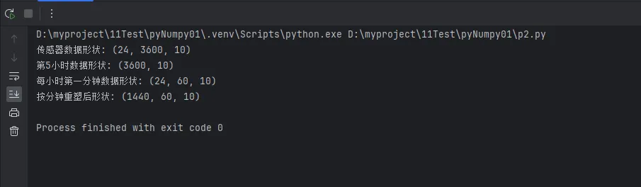
sensor_data = np.random.normal(25, 5, (24, 3600, 10)) # 24小时 × 3600秒 × 10个点
print(f"传感器数据形状: {sensor_data.shape}")
# 需求:提取第5小时的所有数据 - 这需要索引技能
hour_5_data = sensor_data[4] # 索引从0开始
print(f"第5小时数据形状: {hour_5_data.shape}")
# 需求:提取每小时的第一分钟数据 - 这需要切片技能
first_minute_data = sensor_data[:, :60, :]
print(f"每小时第一分钟数据形状: {first_minute_data.shape}")
# 需求:将数据重塑为按分钟统计 - 这需要形状变换技能
minute_data = sensor_data.reshape(24*60, 60, 10)
print(f"按分钟重塑后形状: {minute_data.shape}")
这个简单的例子展示了为什么这三项技能在实际项目中缺一不可。
💡 解决方案:数组索引的五种核心技法
🌟 技法一:基础索引 - 精确定位每个元素
基础索引是所有数组操作的基础,必须熟练掌握:
Pythonimport numpy as np
# 创建多维数组用于演示
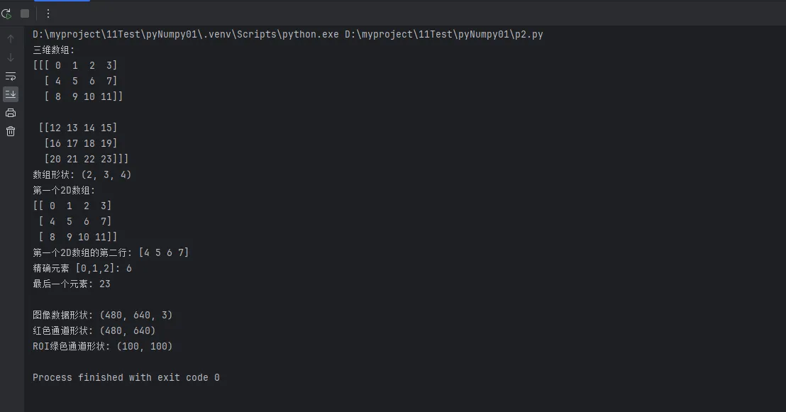
arr_3d = np.arange(24).reshape(2, 3, 4)
print(f"三维数组:\n{arr_3d}")
print(f"数组形状: {arr_3d.shape}")
# 一维索引:提取第一个2D数组
first_2d = arr_3d[0]
print(f"第一个2D数组:\n{first_2d}")
# 二维索引:提取第一个2D数组的第二行
second_row = arr_3d[0, 1]
print(f"第一个2D数组的第二行: {second_row}")
# 三维索引:精确到单个元素
single_element = arr_3d[0, 1, 2]
print(f"精确元素 [0,1,2]: {single_element}")
# 负数索引:从末尾开始计数
last_element = arr_3d[-1, -1, -1]
print(f"最后一个元素: {last_element}")
# Windows环境实战技巧:处理图像数据
# 模拟RGB图像数据 (高度, 宽度, 通道)
image_data = np.random.randint(0, 256, (480, 640, 3), dtype=np.uint8)
print(f"\n图像数据形状: {image_data.shape}")
# 提取红色通道
red_channel = image_data[:, :, 0]
print(f"红色通道形状: {red_channel.shape}")
# 提取左上角100x100像素区域的绿色通道
roi_green = image_data[:100, :100, 1]
print(f"ROI绿色通道形状: {roi_green.shape}")
实战经验:在Windows下处理图像或传感器数据时,始终记住数组的维度顺序,这能避免90%的索引错误。
🌟 技法二:切片操作 - 批量数据提取的艺术
切片操作是NumPy最强大的功能之一,掌握它能大幅提升数据处理效率:
Python# 创建示例数据
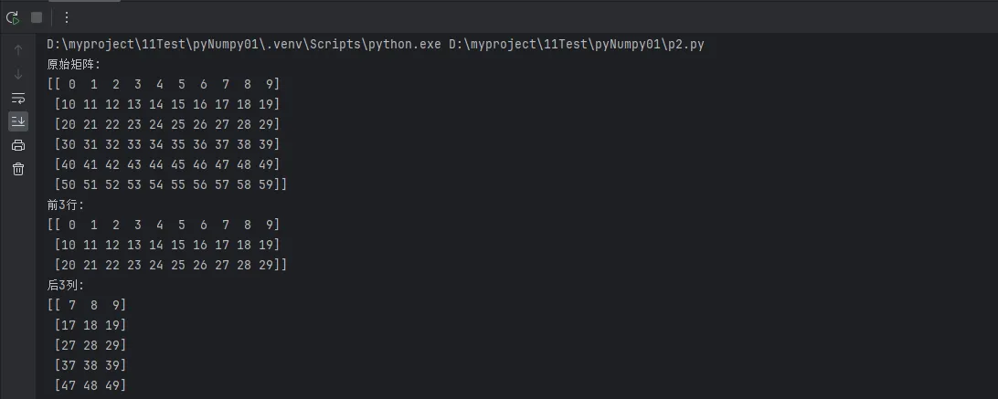
data_matrix = np.arange(60).reshape(6, 10)
print(f"原始矩阵:\n{data_matrix}")
# 基础切片:start:end:step
print(f"前3行: \n{data_matrix[:3]}")
print(f"后3列: \n{data_matrix[:, -3:]}")
print(f"每隔一行: \n{data_matrix[::2]}")
# 高级切片组合
print(f"中间区域 (行1-4, 列2-7):\n{data_matrix[1:5, 2:8]}")
# 实战应用:时间序列数据分析
# 模拟股票价格数据:252个交易日,每日(开盘,最高,最低,收盘,成交量)
stock_data = np.random.random((252, 5)) * 100 + 50
print(f"\n股票数据形状: {stock_data.shape}")
# 提取最近30个交易日的收盘价
recent_close = stock_data[-30:, 3] # 第3列是收盘价
print(f"最近30日收盘价: {recent_close[:5]}...") # 只显示前5个
# 提取每周五的数据(假设从周一开始)
fridays_data = stock_data[4::5] # 从第4个开始,每5个取一个
print(f"周五数据形状: {fridays_data.shape}")
# 提取特定时间段的高低价格
q1_high_low = stock_data[:63, [1, 2]] # 第一季度的最高和最低价
print(f"Q1高低价格形状: {q1_high_low.shape}")
# Windows开发实用技巧:数据窗口提取
def extract_moving_window(data, window_size):
"""
提取移动窗口数据 - 在时间序列分析中常用
"""
result = []
for i in range(len(data) - window_size + 1):
window = data[i:i + window_size]
result.append(window)
return np.array(result)
# 提取5日移动窗口
windows_5d = extract_moving_window(stock_data[:, 3], 5)
print(f"5日移动窗口形状: {windows_5d.shape}")
print(f"第一个窗口: {windows_5d[0]}")
性能提示:使用切片操作比使用循环快50-100倍,这在处理大数据时优势明显。
🌟 技法三:布尔索引 - 条件筛选的利器
布尔索引是数据筛选和条件处理的最佳工具:
Python# 创建测试数据
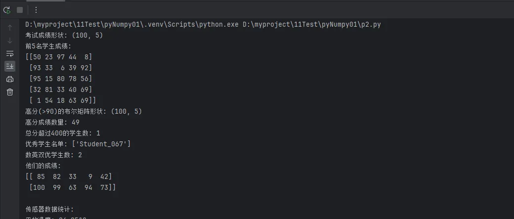
test_scores = np.random.randint(0, 101, (100, 5)) # 100个学生,5门科目
student_names = np.array([f"Student_{i:03d}" for i in range(100)])
print(f"考试成绩形状: {test_scores.shape}")
print(f"前5名学生成绩:\n{test_scores[:5]}")
# 基础布尔索引
high_scores = test_scores > 90
print(f"高分(>90)的布尔矩阵形状: {high_scores.shape}")
print(f"高分成绩数量: {np.sum(high_scores)}")
# 条件筛选:找出总分超过400的学生
total_scores = np.sum(test_scores, axis=1)
high_total_mask = total_scores > 400
high_performers = student_names[high_total_mask]
print(f"总分超过400的学生数: {len(high_performers)}")
print(f"优秀学生名单: {high_performers[:5]}") # 显示前5名
# 复杂条件组合
# 找出数学(第0科)>=85 且 英语(第1科)>=80 的学生
math_english_good = (test_scores[:, 0] >= 85) & (test_scores[:, 1] >= 80)
qualified_students = student_names[math_english_good]
qualified_scores = test_scores[math_english_good]
print(f"数英双优学生数: {len(qualified_students)}")
print(f"他们的成绩:\n{qualified_scores[:3]}")
# 实战应用:传感器数据异常检测
# 模拟温度传感器数据
temperature_data = np.random.normal(25, 3, 1000) # 正常温度分布
# 人为添加一些异常值
anomaly_indices = np.random.choice(1000, 50, replace=False)
temperature_data[anomaly_indices] += np.random.uniform(-15, 15, 50)
print(f"\n传感器数据统计:")
print(f"平均温度: {np.mean(temperature_data):.2f}°C")
print(f"标准差: {np.std(temperature_data):.2f}°C")
# 使用3σ原则检测异常值
mean_temp = np.mean(temperature_data)
std_temp = np.std(temperature_data)
threshold = 3 * std_temp
# 异常值检测
anomaly_mask = np.abs(temperature_data - mean_temp) > threshold
normal_mask = ~anomaly_mask # 取反,得到正常值的掩码
print(f"检测到异常值: {np.sum(anomaly_mask)}个")
print(f"异常温度范围: {temperature_data[anomaly_mask].min():.1f}°C ~ {temperature_data[anomaly_mask].max():.1f}°C")
# 清理异常数据
clean_temperature = temperature_data[normal_mask]
print(f"清理后数据点数: {len(clean_temperature)}")
# Windows开发实用函数:多条件筛选器
def multi_condition_filter(data, conditions):
"""
多条件数据筛选器
conditions: list of (column_index, operator, value) tuples
"""
mask = np.ones(len(data), dtype=bool) # 初始全为True
for col_idx, operator, value in conditions:
if operator == '>':
mask &= (data[:, col_idx] > value)
elif operator == '<':
mask &= (data[:, col_idx] < value)
elif operator == '>=':
mask &= (data[:, col_idx] >= value)
elif operator == '<=':
mask &= (data[:, col_idx] <= value)
elif operator == '==':
mask &= (data[:, col_idx] == value)
return data[mask], mask
# 使用多条件筛选器
conditions = [
(0, '>=', 80), # 第0科 >= 80
(1, '>=', 75), # 第1科 >= 75
(4, '<', 95) # 第4科 < 95
]
filtered_scores, filter_mask = multi_condition_filter(test_scores, conditions)
filtered_students = student_names[filter_mask]
print(f"\n多条件筛选结果:")
print(f"符合条件的学生数: {len(filtered_students)}")
print(f"筛选比例: {len(filtered_students)/len(student_names)*100:.1f}%")
编程技巧:在Windows环境下处理大数据时,布尔索引比使用pandas的query方法更高效,内存占用也更少。
🌟 技法四:花式索引 - 非连续数据的精确提取
花式索引允许我们使用数组作为索引,实现复杂的数据提取:
Python# 创建示例数据矩阵
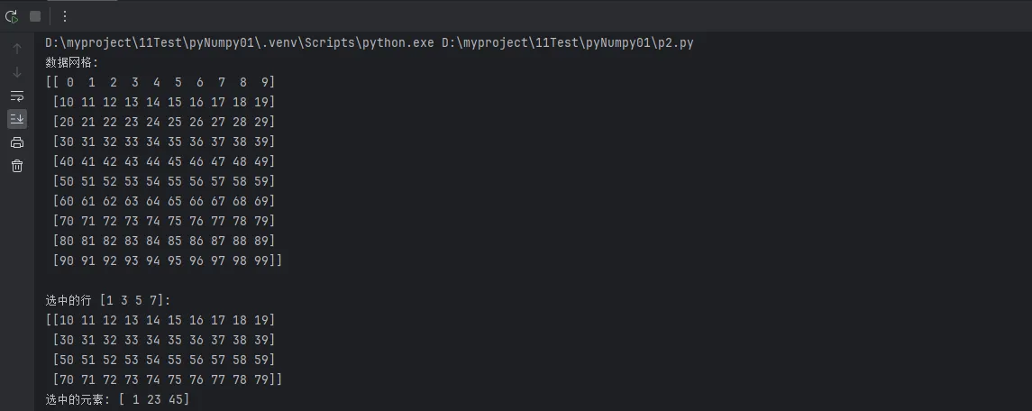
data_grid = np.arange(100).reshape(10, 10)
print(f"数据网格:\n{data_grid}")
# 基础花式索引:使用数组作为索引
row_indices = np.array([1, 3, 5, 7])
selected_rows = data_grid[row_indices]
print(f"\n选中的行 {row_indices}:\n{selected_rows}")
# 同时指定行和列索引
row_idx = np.array([0, 2, 4])
col_idx = np.array([1, 3, 5])
selected_elements = data_grid[row_idx, col_idx] # 提取(0,1), (2,3), (4,5)的元素
print(f"选中的元素: {selected_elements}")
# 实战应用:用户行为分析
# 模拟用户访问数据:100个用户,30天的访问次数
user_visits = np.random.poisson(5, (100, 30)) # 泊松分布,平均5次访问
print(f"\n用户访问数据形状: {user_visits.shape}")
# 找出最活跃的10个用户
total_visits = np.sum(user_visits, axis=1)
top_users_idx = np.argsort(total_visits)[-10:] # 最大的10个索引
top_users_visits = user_visits[top_users_idx]
print(f"最活跃10用户的总访问次数: {total_visits[top_users_idx]}")
# 提取特定日期的数据(比如周末)
weekend_days = np.array([5, 6, 12, 13, 19, 20, 26, 27]) # 假设这些是周末
weekend_visits = user_visits[:, weekend_days]
print(f"周末访问数据形状: {weekend_visits.shape}")
# 高级应用:基于排序的采样
# 对每个用户按访问量排序,提取访问量最高的5天
def top_days_per_user(visit_data, top_n=5):
"""为每个用户找出访问量最高的N天"""
result = np.zeros((len(visit_data), top_n))
day_indices = np.zeros((len(visit_data), top_n), dtype=int)
for i, user_data in enumerate(visit_data):
# 获取该用户访问量最高的top_n天的索引
top_day_idx = np.argsort(user_data)[-top_n:]
day_indices[i] = top_day_idx
result[i] = user_data[top_day_idx]
return result, day_indices
top_visit_data, top_day_indices = top_days_per_user(user_visits)
print(f"每用户最活跃5天的访问数据形状: {top_visit_data.shape}")
print(f"第一个用户最活跃的5天: 第{top_day_indices[0]}天")
# Windows开发实用技巧:批量数据重排
def reorder_by_priority(data, priority_indices):
"""
根据优先级索引重新排列数据
常用于任务调度、数据重组等场景
"""
if len(priority_indices) != len(data):
raise ValueError("优先级索引长度必须与数据长度相同")
return data[priority_indices]
# 模拟任务优先级调度
task_data = np.random.randint(1, 100, (20, 4)) # 20个任务,4个属性
task_priorities = np.random.rand(20) # 随机优先级
# 按优先级排序
priority_order = np.argsort(task_priorities)[::-1] # 降序排列
sorted_tasks = reorder_by_priority(task_data, priority_order)
print(f"\n任务调度示例:")
print(f"原始任务数据形状: {task_data.shape}")
print(f"按优先级排序后前3个任务:\n{sorted_tasks[:3]}")
实战技巧:花式索引在处理稀疏数据和非规律采样时特别有用,是数据科学项目的常用技能。
🌟 技法五:组合索引 - 复杂数据提取的终极技法
组合索引将前面所有技法整合,应对最复杂的数据提取需求:
Python# 创建复杂的多维数据集
# 模拟一个小型ERP系统的销售数据
# 维度:[月份(12), 产品类别(5), 销售指标(4: 销量,金额,成本,利润)]
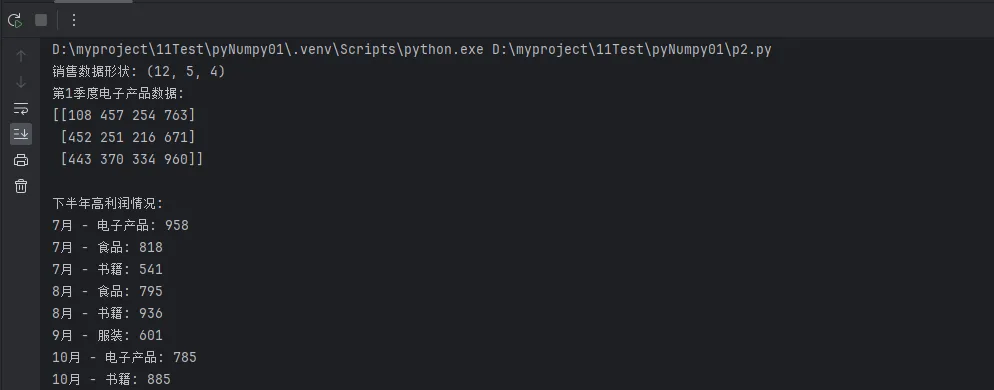
sales_data = np.random.randint(100, 1000, (12, 5, 4))
# 添加一些标签方便理解
months = ['1月', '2月', '3月', '4月', '5月', '6月', '7月', '8月', '9月', '10月', '11月', '12月']
categories = ['电子产品', '服装', '食品', '书籍', '家具']
metrics = ['销量', '金额', '成本', '利润']
print(f"销售数据形状: {sales_data.shape}")
print(f"第1季度电子产品数据:\n{sales_data[:3, 0, :]}")
# 组合技法1:切片 + 布尔索引
# 找出下半年(7-12月)利润超过500的产品类别和月份
second_half = sales_data[6:] # 下半年数据
profit_data = second_half[:, :, 3] # 利润数据
high_profit_mask = profit_data > 500
# 找出高利润的月份和产品
high_profit_months, high_profit_categories = np.where(high_profit_mask)
high_profit_months += 6 # 调整为实际月份索引
print(f"\n下半年高利润情况:")
for i in range(len(high_profit_months)):
month_idx = high_profit_months[i]
cat_idx = high_profit_categories[i]
profit_value = sales_data[month_idx, cat_idx, 3]
print(f"{months[month_idx]} - {categories[cat_idx]}: {profit_value}")
# 组合技法2:花式索引 + 切片
# 提取特定月份的特定产品的完整数据
target_months = [0, 3, 6, 9] # 每季度第一个月
target_categories = [0, 2, 4] # 电子产品、食品、家具
quarterly_data = sales_data[np.ix_(target_months, target_categories)]
print(f"\n季度特定产品数据形状: {quarterly_data.shape}")
# 组合技法3:复杂条件筛选
# 找出销量>300 且 利润>400 的所有记录
volume_condition = sales_data[:, :, 0] > 300 # 销量条件
profit_condition = sales_data[:, :, 3] > 400 # 利润条件
combined_condition = volume_condition & profit_condition
# 提取满足条件的完整记录
good_performance_months, good_performance_categories = np.where(combined_condition)
print(f"\n高效益记录数量: {len(good_performance_months)}")
# Windows实战应用:数据报表生成器
class SalesReportGenerator:
"""销售数据报表生成器 - Windows环境下的实用工具类"""
def __init__(self, sales_data, months, categories, metrics):
self.sales_data = sales_data
self.months = months
self.categories = categories
self.metrics = metrics
def monthly_summary(self, month_idx):
"""生成月度汇总报表"""
month_data = self.sales_data[month_idx]
print(f"\n=== {self.months[month_idx]}销售汇总 ===")
for i, category in enumerate(self.categories):
print(f"{category}:")
for j, metric in enumerate(self.metrics):
print(f" {metric}: {month_data[i, j]}")
def category_trend(self, category_idx):
"""生成产品类别趋势报表"""
category_data = self.sales_data[:, category_idx, :]
print(f"\n=== {self.categories[category_idx]}年度趋势 ===")
for i, month in enumerate(self.months):
profit_margin = (category_data[i, 3] / category_data[i, 1] * 100
if category_data[i, 1] > 0 else 0)
print(f"{month}: 利润率 {profit_margin:.1f}%")
def top_performers(self, metric_idx, top_n=5):
"""找出指定指标的Top N表现"""
metric_data = self.sales_data[:, :, metric_idx]
# 展平数据并找出最大值的索引
flat_data = metric_data.flatten()
top_indices = np.argsort(flat_data)[-top_n:][::-1]
# 转换回二维索引
month_indices, cat_indices = np.unravel_index(top_indices, metric_data.shape)
print(f"\n=== {self.metrics[metric_idx]}Top {top_n} ===")
for i in range(top_n):
month_idx = month_indices[i]
cat_idx = cat_indices[i]
value = self.sales_data[month_idx, cat_idx, metric_idx]
print(f"第{i+1}名: {self.months[month_idx]} - {self.categories[cat_idx]} - {value}")
# 使用报表生成器
report_gen = SalesReportGenerator(sales_data, months, categories, metrics)
report_gen.monthly_summary(0) # 1月汇总
report_gen.category_trend(0) # 电子产品趋势
report_gen.top_performers(3) # 利润Top 5
🔄 形状操作:数据结构变换的艺术
reshape:最常用的形状变换
Python# 基础reshape操作
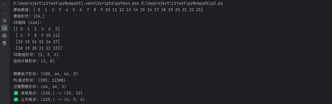
original_array = np.arange(24)
print(f"原始数组: {original_array}")
print(f"原始形状: {original_array.shape}")
# 变换为不同形状
matrix_2d = original_array.reshape(4, 6)
print(f"2D矩阵 (4x6):\n{matrix_2d}")
matrix_3d = original_array.reshape(2, 3, 4)
print(f"3D数组形状: {matrix_3d.shape}")
# 使用-1让NumPy自动计算维度
auto_reshape = original_array.reshape(3, -1) # 自动计算第二维
print(f"自动计算形状: {auto_reshape.shape}")
# 实战应用:图像数据处理
# 模拟彩色图像数据:100张 64x64 RGB图像
image_batch = np.random.randint(0, 256, (100, 64, 64, 3))
print(f"\n图像批次形状: {image_batch.shape}")
# 重塑为机器学习友好的格式
ml_format = image_batch.reshape(100, -1) # 每张图像展平为一维
print(f"ML格式形状: {ml_format.shape}")
# 将单张图像重塑回原始格式
single_image = ml_format[0].reshape(64, 64, 3)
print(f"还原图像形状: {single_image.shape}")
# Windows开发实用技巧:批处理数据重整
def batch_reshape_processor(data_batch, target_shapes):
"""
批量重塑数据处理器
适用于需要将同一批数据变换为多种形状的场景
"""
results = {}
for name, shape in target_shapes.items():
try:
results[name] = data_batch.reshape(shape)
print(f"✅ {name}: {data_batch.shape} -> {shape}")
except ValueError as e:
print(f"❌ {name}: 重塑失败 - {e}")
return results
# 使用批处理重塑器
test_data = np.arange(120)
target_formats = {
'表格格式': (10, 12),
'立方格式': (4, 5, 6),
'时序格式': (24, 5),
'错误格式': (7, 11) # 故意设置错误以演示错误处理
}
reshaped_results = batch_reshape_processor(test_data, target_formats)
转置与轴交换
Python# 创建示例矩阵
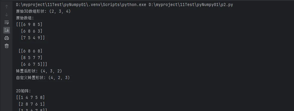
matrix_3d = np.random.randint(1, 10, (2, 3, 4))
print(f"原始3D数组形状: {matrix_3d.shape}")
print(f"原始数组:\n{matrix_3d}")
# 基础转置
transposed = matrix_3d.transpose()
print(f"转置后形状: {transposed.shape}")
# 指定轴的转置
custom_transpose = matrix_3d.transpose(2, 0, 1) # (2,3,4) -> (4,2,3)
print(f"自定义转置形状: {custom_transpose.shape}")
# 2D矩阵转置的简便方法
matrix_2d = np.random.randint(1, 10, (3, 5))
print(f"\n2D矩阵:\n{matrix_2d}")
print(f"转置矩阵:\n{matrix_2d.T}")
# 实战应用:数据表格行列转换
# 模拟销售数据:5个销售员,12个月的业绩
sales_by_person = np.random.randint(1000, 5000, (5, 12))
print(f"\n按销售员组织的数据形状: {sales_by_person.shape}")
# 转换为按月份组织
sales_by_month = sales_by_person.T
print(f"按月份组织的数据形状: {sales_by_month.shape}")
# 轴交换:swapaxes
data_3d = np.random.randint(1, 100, (10, 20, 30))
print(f"\n原始数据形状: {data_3d.shape}")
# 交换第0轴和第2轴
swapped = np.swapaxes(data_3d, 0, 2)
print(f"轴交换后形状: {swapped.shape}")
# Windows实战:数据维度适配器
class DimensionAdapter:
"""数据维度适配器 - 用于不同数据格式间的转换"""
@staticmethod
def image_format_converter(images, source_format, target_format):
"""
图像格式转换器
支持的格式:
- 'HWC': Height-Width-Channel
- 'CHW': Channel-Height-Width
- 'NHWC': Batch-Height-Width-Channel
- 'NCHW': Batch-Channel-Height-Width
"""
format_axes = {
'HWC': (0, 1, 2),
'CHW': (2, 0, 1),
'NHWC': (0, 1, 2, 3),
'NCHW': (0, 3, 1, 2)
}
if source_format == target_format:
return images
# 定义转换映射
conversions = {
('NHWC', 'NCHW'): (0, 3, 1, 2),
('NCHW', 'NHWC'): (0, 2, 3, 1),
('HWC', 'CHW'): (2, 0, 1),
('CHW', 'HWC'): (1, 2, 0)
}
conversion_key = (source_format, target_format)
if conversion_key in conversions:
return images.transpose(conversions[conversion_key])
else:
raise ValueError(f"不支持从{source_format}到{target_format}的转换")
# 使用维度适配器
sample_images_nhwc = np.random.randint(0, 256, (32, 224, 224, 3)) # 批次格式
print(f"NHWC格式: {sample_images_nhwc.shape}")
sample_images_nchw = DimensionAdapter.image_format_converter(
sample_images_nhwc, 'NHWC', 'NCHW'
)
print(f"NCHW格式: {sample_images_nchw.shape}")
数组拼接与分割
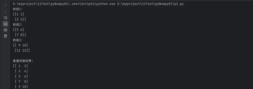
Python# 创建示例数组
arr1 = np.array([[1, 2], [3, 4]])
arr2 = np.array([[5, 6], [7, 8]])
arr3 = np.array([[9, 10], [11, 12]])

print(f"数组1:\n{arr1}")
print(f"数组2:\n{arr2}")
print(f"数组3:\n{arr3}")

# 垂直拼接(增加行)
v_concat = np.vstack([arr1, arr2, arr3])
print(f"\n垂直拼接结果:\n{v_concat}")
print(f"拼接后形状: {v_concat.shape}")

# 水平拼接(增加列)
h_concat = np.hstack([arr1, arr2, arr3])
print(f"\n水平拼接结果:\n{h_concat}")
print(f"拼接后形状: {h_concat.shape}")

# 通用拼接函数
concat_axis0 = np.concatenate([arr1, arr2, arr3], axis=0)
concat_axis1 = np.concatenate([arr1, arr2, arr3], axis=1)

print(f"\naxis=0拼接等同于vstack: {np.array_equal(concat_axis0, v_concat)}")
print(f"axis=1拼接等同于hstack: {np.array_equal(concat_axis1, h_concat)}")

# 数组分割
large_array = np.arange(24).reshape(6, 4)
print(f"\n原始大数组:\n{large_array}")

# 等分割
v_splits = np.vsplit(large_array, 3)  # 垂直分为3部分
print(f"垂直分割为3部分,第一部分:\n{v_splits[0]}")

h_splits = np.hsplit(large_array, 2)  # 水平分为2部分
print(f"水平分割为2部分,第一部分:\n{h_splits[0]}")

# 不等分割
unequal_splits = np.split(large_array, [2, 5], axis=0)  # 在索引2和5处分割
print(f"不等分割结果数量: {len(unequal_splits)}")
print(f"第一部分形状: {unequal_splits[0].shape}")
print(f"第二部分形状: {unequal_splits[1].shape}")
print(f"第三部分形状: {unequal_splits[2].shape}")

# 实战应用:数据预处理流水线
class DataPreprocessor:
    """数据预处理流水线 - Windows环境下的实用工具"""

    def __init__(self):
        self.processed_data = None

    def load_and_merge_datasets(self, datasets):
        """加载并合并多个数据集"""
        print("📥 加载数据集...")
        merged_data = np.concatenate(datasets, axis=0)
        print(f"✅ 合并完成,最终形状: {merged_data.shape}")
        return merged_data

    def train_test_split(self, data, train_ratio=0.8):
        """分割训练集和测试集"""
        n_samples = len(data)
        split_idx = int(n_samples * train_ratio)

        # 随机打乱数据
        indices = np.random.permutation(n_samples)
        shuffled_data = data[indices]

        # 分割数据
        train_data = shuffled_data[:split_idx]
        test_data = shuffled_data[split_idx:]

        print(f"📊 数据分割完成:")
        print(f"  训练集: {train_data.shape}")
        print(f"  测试集: {test_data.shape}")

        return train_data, test_data

    def create_batches(self, data, batch_size):
        """创建训练批次"""
        n_samples = len(data)
        n_batches = (n_samples + batch_size - 1) // batch_size

        batches = []
        for i in range(n_batches):
            start_idx = i * batch_size
            end_idx = min((i + 1) * batch_size, n_samples)
            batch = data[start_idx:end_idx]
            batches.append(batch)

        print(f"🔄 创建批次完成:")
        print(f"  批次数量: {len(batches)}")
        print(f"  批次大小: {batch_size}")

        return batches

# 使用数据预处理流水线
preprocessor = DataPreprocessor()

# 模拟多个数据集
dataset1 = np.random.random((1000, 10))
dataset2 = np.random.random((800, 10))
dataset3 = np.random.random((1200, 10))

# 执行预处理流水线
merged_data = preprocessor.load_and_merge_datasets([dataset1, dataset2, dataset3])
train_data, test_data = preprocessor.train_test_split(merged_data)
train_batches = preprocessor.create_batches(train_data, batch_size=128)

print(f"\n🎯 预处理完成!")
print(f"训练批次示例形状: {train_batches[0].shape}")
⚡ 性能优化与最佳实践
Python# 性能优化技巧汇总
import time
import numpy as np
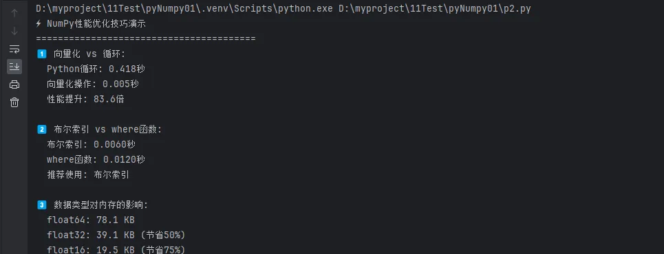
def performance_comparison():
"""性能对比测试"""
print("⚡ NumPy性能优化技巧演示")
print("=" * 40)
# 创建大数据集
large_data = np.random.random((1000, 1000))
# 技巧1: 使用向量化操作代替循环
print("1️⃣ 向量化 vs 循环:")
# 错误方式:Python循环
start = time.time()
result_slow = np.zeros_like(large_data)
for i in range(large_data.shape[0]):
for j in range(large_data.shape[1]):
result_slow[i, j] = large_data[i, j] ** 2 + 1
time_slow = time.time() - start
# 正确方式:向量化操作
start = time.time()
result_fast = large_data ** 2 + 1
time_fast = time.time() - start
print(f" Python循环: {time_slow:.3f}秒")
print(f" 向量化操作: {time_fast:.3f}秒")
print(f" 性能提升: {time_slow/time_fast:.1f}倍")
# 技巧2: 布尔索引 vs where函数
print("\n2️⃣ 布尔索引 vs where函数:")
# 布尔索引
start = time.time()
mask = large_data > 0.5
filtered_bool = large_data[mask]
time_bool = time.time() - start
# where函数
start = time.time()
indices = np.where(large_data > 0.5)
filtered_where = large_data[indices]
time_where = time.time() - start
print(f" 布尔索引: {time_bool:.4f}秒")
print(f" where函数: {time_where:.4f}秒")
print(f" 推荐使用: {'布尔索引' if time_bool < time_where else 'where函数'}")
# 技巧3: 合理选择数据类型
print("\n3️⃣ 数据类型对内存的影响:")
# 不同精度的数组
array_f64 = np.random.random(10000).astype(np.float64)
array_f32 = array_f64.astype(np.float32)
array_f16 = array_f64.astype(np.float16)
print(f" float64: {array_f64.nbytes / 1024:.1f} KB")
print(f" float32: {array_f32.nbytes / 1024:.1f} KB (节省{(1-array_f32.nbytes/array_f64.nbytes)*100:.0f}%)")
print(f" float16: {array_f16.nbytes / 1024:.1f} KB (节省{(1-array_f16.nbytes/array_f64.nbytes)*100:.0f}%)")
performance_comparison()
🎯 结尾呼应
通过本文的深入学习,我们已经完全掌握了NumPy数组索引、切片与形状操作的精髓。让我们来总结三个最关键的要点:
1. 索引和切片是数据提取的核心技能:从基础的单元素索引到复杂的布尔索引,从简单的切片到花式索引的组合应用,这些技能构成了数据处理的基础。在Windows环境下进行Python开发时,熟练掌握这些操作能让你轻松应对各种数据提取需求,无论是处理传感器数据、分析日志文件,还是进行图像处理,都能游刃有余。
2. 形状操作是数据适配的关键工具:reshape、transpose、拼接与分割等操作看似简单,实际上是连接不同数据处理环节的桥梁。它们让你能够灵活地在不同的数据格式间转换,适应各种算法和库的输入要求。这种适配能力在实际项目中价值巨大,特别是在需要整合多个数据源或与不同的机器学习框架协作时。
3. 性能优化思维是专业开发的标志:理解向量化操作的优势,合理选择数据类型,善用NumPy的内置函数,这些不仅仅是编程技巧,更是专业开发者的思维方式。在处理大规模数据时,这些优化技巧往往能带来数十倍甚至百倍的性能提升,这种差异在生产环境中是决定性的。
掌握了这些核心技能后,你已经具备了处理复杂数据分析任务的能力。继续深入学习NumPy的线性代数运算、统计函数、以及与其他科学计算库的协作,将让你在Python开发的道路上更进一步。记住,熟能生巧,多在实际项目中应用这些技能,才能真正将知识转化为实战能力。
本文涵盖了NumPy数组操作的核心技能,建议配合实际项目练习。在Windows环境下的开发过程中,这些技能将成为你最得力的工具。如有疑问或需要更深入的讨论,欢迎交流!
本文作者:技术老小子
本文链接:
版权声明:本博客所有文章除特别声明外,均采用 BY-NC-SA 许可协议。转载请注明出处!