
目录
作为Python开发者,你是否在处理数值计算时遇到过性能瓶颈?是否为复杂的数学运算而苦恼?NumPy的数学函数模块正是解决这些问题的利器。本文将从实际开发角度出发,深入剖析NumPy数学函数的核心功能,通过丰富的代码实例,帮助你掌握高效的数值计算技巧。无论你是数据分析新手,还是希望提升计算性能的资深开发者,这篇文章都将为你的Python开发之路提供强有力的支持。
🔍 问题分析:为什么选择NumPy数学函数?
在日常的Python开发中,我们经常遇到以下挑战:
📊 性能瓶颈问题
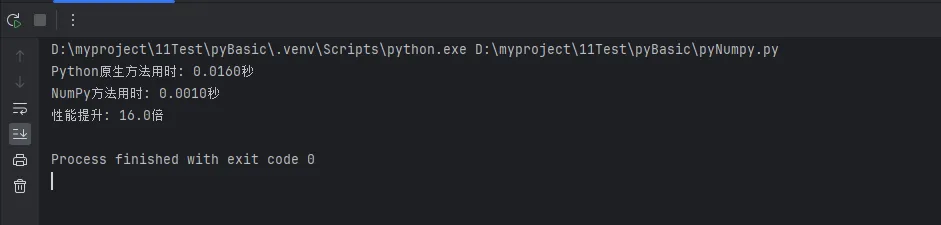
Python原生的math模块虽然功能完整,但在处理大量数据时性能表现不佳:
Pythonimport math
import time
import numpy as np

# 原生Python方法处理10万个数据
data_list = list(range(100000))
start_time = time.time()
result_python = [math.sin(x) for x in data_list]
python_time = time.time() - start_time

# NumPy方法处理相同数据
data_array = np.array(data_list)
start_time = time.time()
result_numpy = np.sin(data_array)
numpy_time = time.time() - start_time

print(f"Python原生方法用时: {python_time:.4f}秒")
print(f"NumPy方法用时: {numpy_time:.4f}秒")
print(f"性能提升: {python_time/numpy_time:.1f}倍")
🎯 功能局限性
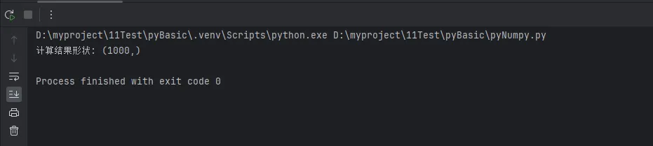
原生Python在处理多维数组运算时代码复杂,而NumPy提供了更优雅的解决方案:
Pythonimport numpy as np

# 复杂的多维数学运算
matrix_2d = np.random.rand(1000, 1000)

# NumPy一行代码完成复杂运算
result = np.sqrt(np.sum(np.square(matrix_2d), axis=1))
print(f"计算结果形状: {result.shape}")
💡 解决方案:NumPy数学函数全景图
NumPy数学函数按功能可以分为以下几大类:
🧮 基础数学运算函数
算术运算
Pythonimport numpy as np
# 创建测试数据
arr = np.array([1, 4, 9, 16, 25])
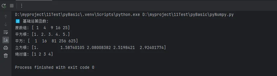
print("🔢 基础运算函数:")
print(f"原数组: {arr}")
print(f"平方根: {np.sqrt(arr)}")
print(f"平方: {np.square(arr)}")
print(f"立方根: {np.cbrt(arr)}")
print(f"绝对值: {np.abs(np.array([-1, -2, 3, -4]))}")
指数与对数
Pythonimport numpy as np
# 指数对数运算
x = np.array([1, 2, 3, 4, 5])
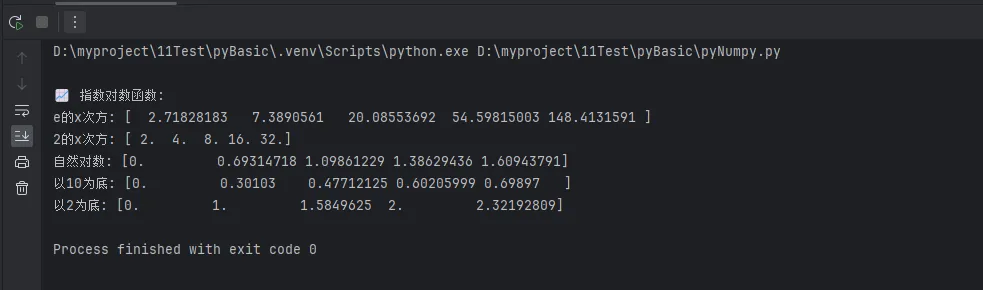
print("\n📈 指数对数函数:")
print(f"e的x次方: {np.exp(x)}")
print(f"2的x次方: {np.exp2(x)}")
print(f"自然对数: {np.log(x)}")
print(f"以10为底: {np.log10(x)}")
print(f"以2为底: {np.log2(x)}")
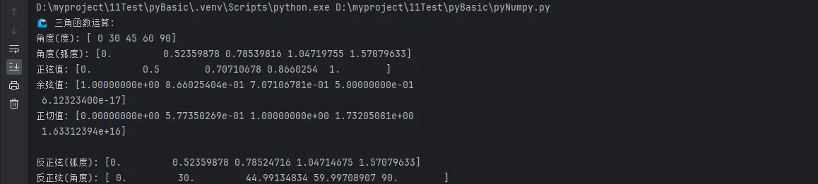
🌊 三角函数与反三角函数
三角函数在上位机开发中的信号处理和图形绘制中应用广泛:
Pythonimport numpy as np

# 角度转弧度
angles_deg = np.array([0, 30, 45, 60, 90])
angles_rad = np.deg2rad(angles_deg)

print("🌊 三角函数运算:")
print(f"角度(度): {angles_deg}")
print(f"角度(弧度): {angles_rad}")
print(f"正弦值: {np.sin(angles_rad)}")
print(f"余弦值: {np.cos(angles_rad)}")
print(f"正切值: {np.tan(angles_rad)}")

# 反三角函数
sin_values = np.array([0, 0.5, 0.707, 0.866, 1])
print(f"\n反正弦(弧度): {np.arcsin(sin_values)}")
print(f"反正弦(角度): {np.rad2deg(np.arcsin(sin_values))}")
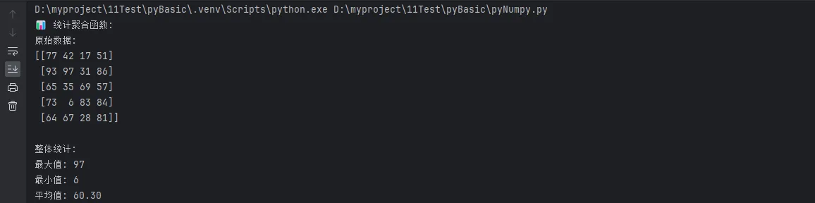
📊 统计与聚合函数
在数据分析中,这些函数是必不可少的工具:
Pythonimport numpy as np

# 创建二维测试数据
data_2d = np.random.randint(1, 100, (5, 4))
print("📊 统计聚合函数:")
print(f"原始数据:\n{data_2d}")

print(f"\n整体统计:")
print(f"最大值: {np.max(data_2d)}")
print(f"最小值: {np.min(data_2d)}")
print(f"平均值: {np.mean(data_2d):.2f}")
print(f"标准差: {np.std(data_2d):.2f}")
print(f"方差: {np.var(data_2d):.2f}")

print(f"\n按轴统计:")
print(f"每列最大值: {np.max(data_2d, axis=0)}")
print(f"每行平均值: {np.round(np.mean(data_2d, axis=1), 2)}")
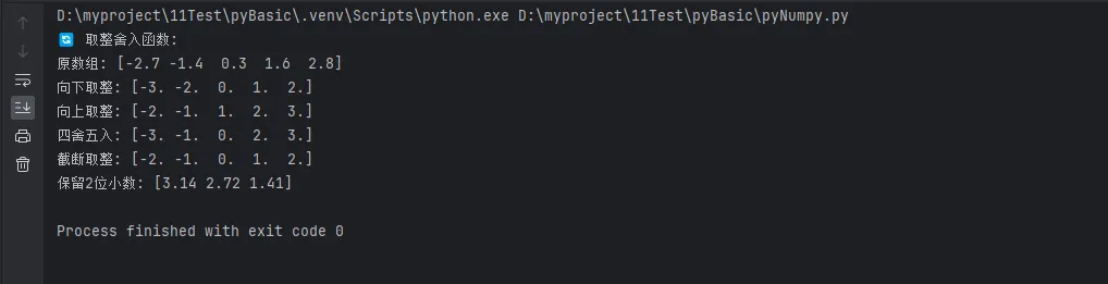
🔄 取整与舍入函数
精确控制数值精度在金融计算和工程应用中至关重要:
Pythonimport numpy as np

decimal_array = np.array([-2.7, -1.4, 0.3, 1.6, 2.8])

print("🔄 取整舍入函数:")
print(f"原数组: {decimal_array}")
print(f"向下取整: {np.floor(decimal_array)}")
print(f"向上取整: {np.ceil(decimal_array)}")
print(f"四舍五入: {np.round(decimal_array)}")
print(f"截断取整: {np.trunc(decimal_array)}")

# 控制小数位数
precise_array = np.array([3.14159, 2.71828, 1.41421])
print(f"保留2位小数: {np.round(precise_array, 2)}")
🔧 代码实战:实际应用场景
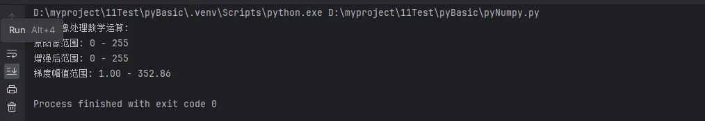
🎨 场景一:图像处理中的数学运算
在Python开发的图像处理项目中,NumPy数学函数发挥重要作用:
Pythonimport numpy as np


def image_enhancement_demo():
    """图像增强示例"""
    # 模拟灰度图像数据 (0-255)
    image = np.random.randint(0, 256, (100, 100), dtype=np.uint8)

    print("🎨 图像处理数学运算:")
    print(f"原图像范围: {image.min()} - {image.max()}")

    # 对比度增强 - 使用指数运算
    enhanced = np.power(image / 255.0, 0.7) * 255
    enhanced = np.clip(enhanced, 0, 255).astype(np.uint8)
    print(f"增强后范围: {enhanced.min()} - {enhanced.max()}")

    # 边缘检测预处理 - 使用梯度运算
    grad_x = np.diff(image.astype(np.float32), axis=1)
    grad_y = np.diff(image.astype(np.float32), axis=0)

    # 梯度幅值 (修复形状不匹配问题)
    gradient_magnitude = np.sqrt(grad_x[:-1, :] ** 2 + grad_y[:, :-1] ** 2)
    print(f"梯度幅值范围: {gradient_magnitude.min():.2f} - {gradient_magnitude.max():.2f}")

    return enhanced, gradient_magnitude


# 运行演示
enhanced_img, grad_img = image_enhancement_demo()
📈 场景二:金融数据分析
编程技巧在量化分析中的应用:
Pythonimport numpy as np
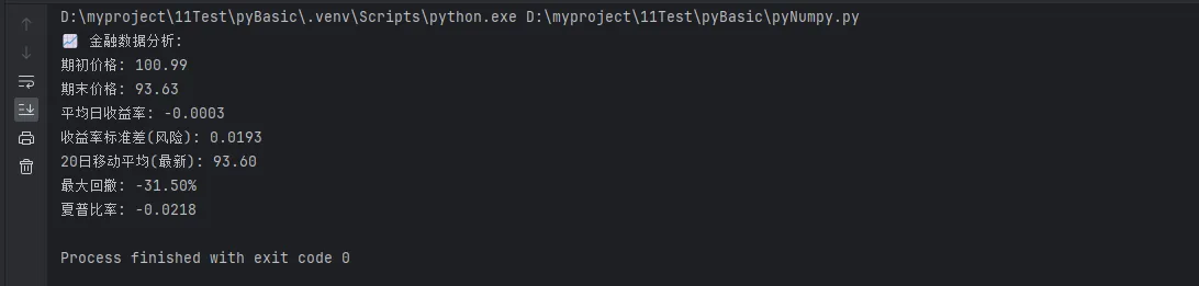
def financial_analysis_demo():
"""金融数据分析示例"""
# 模拟股价数据
np.random.seed(42)
price_changes = np.random.normal(0, 0.02, 252) # 一年的交易日
prices = np.cumprod(1 + price_changes) * 100 # 从100开始的价格序列
print("📈 金融数据分析:")
print(f"期初价格: {prices[0]:.2f}")
print(f"期末价格: {prices[-1]:.2f}")
# 计算收益率
returns = np.diff(np.log(prices))
print(f"平均日收益率: {np.mean(returns):.4f}")
print(f"收益率标准差(风险): {np.std(returns):.4f}")
# 计算移动平均线
window = 20
ma_20 = np.convolve(prices, np.ones(window) / window, mode='valid')
print(f"20日移动平均(最新): {ma_20[-1]:.2f}")
# 计算最大回撤
peak = np.maximum.accumulate(prices)
drawdown = (prices - peak) / peak
max_drawdown = np.min(drawdown)
print(f"最大回撤: {max_drawdown:.2%}")
# 夏普比率 (假设无风险利率为3%)
rf_rate = 0.03 / 252 # 日无风险利率
sharpe_ratio = (np.mean(returns) - rf_rate) / np.std(returns)
print(f"夏普比率: {sharpe_ratio:.4f}")
# 运行分析
financial_analysis_demo()
🔬 场景三:科学计算中的复杂函数
高级数学函数在科学研究中的应用:
Pythonimport numpy as np
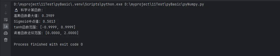
def scientific_computing_demo():
"""科学计算示例"""
x = np.linspace(-5, 5, 1000)
print("🔬 科学计算函数:")
# 高斯函数 (正态分布概率密度函数)
gaussian = np.exp(-0.5 * x ** 2) / np.sqrt(2 * np.pi)
print(f"高斯函数最大值: {np.max(gaussian):.4f}")
# Sigmoid函数 (神经网络激活函数)
sigmoid = 1 / (1 + np.exp(-x))
print(f"Sigmoid中点值: {sigmoid[len(sigmoid) // 2]:.4f}")
# 双曲函数
sinh_vals = np.sinh(x)
cosh_vals = np.cosh(x)
tanh_vals = np.tanh(x)
print(f"tanh函数范围: [{np.min(tanh_vals):.4f}, {np.max(tanh_vals):.4f}]")
# 特殊函数 - 误差函数 (需要scipy,这里用近似)
# 近似误差函数
erf_approx = 2 / np.sqrt(np.pi) * np.cumsum(np.exp(-x ** 2)) * (x[1] - x[0])
print(f"误差函数近似范围: [{np.min(erf_approx):.4f}, {np.max(erf_approx):.4f}]")
return x, gaussian, sigmoid, tanh_vals
# 运行科学计算演示
x_vals, gauss, sigm, tanh = scientific_computing_demo()
⚡ 场景四:性能优化实战
大数据量处理的编程技巧:
Pythonimport time
import numpy as np
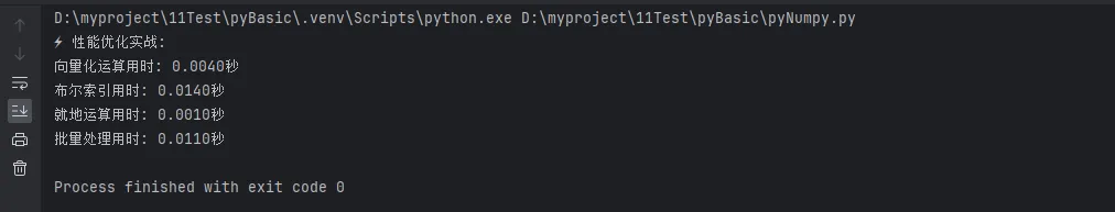
def performance_optimization_demo():
"""性能优化演示"""
# 创建大型数据集
large_data = np.random.randn(1000000)
print("⚡ 性能优化实战:")
# 方法1:使用NumPy向量化运算
start_time = time.time()
result1 = np.sqrt(np.clip(large_data, 0, None))
time1 = time.time() - start_time
print(f"向量化运算用时: {time1:.4f}秒")
# 方法2:使用布尔索引
start_time = time.time()
result2 = np.zeros_like(large_data)
mask = large_data > 0
result2[mask] = np.sqrt(large_data[mask])
time2 = time.time() - start_time
print(f"布尔索引用时: {time2:.4f}秒")
# 内存使用优化 - 就地运算
data_copy = large_data.copy()
start_time = time.time()
np.clip(data_copy, -2, 2, out=data_copy) # 就地修改
time3 = time.time() - start_time
print(f"就地运算用时: {time3:.4f}秒")
# 批量处理大数据
def batch_process(data, batch_size=10000):
results = []
for i in range(0, len(data), batch_size):
batch = data[i:i + batch_size]
processed = np.exp(np.clip(batch, -10, 10)) # 避免溢出
results.append(processed)
return np.concatenate(results)
start_time = time.time()
batch_result = batch_process(large_data)
time4 = time.time() - start_time
print(f"批量处理用时: {time4:.4f}秒")
return time1, time2, time3, time4
# 运行性能测试
times = performance_optimization_demo()
🛠️ 高级技巧与最佳实践
🎯 数值稳定性处理
在实际的Python开发中,数值稳定性是一个重要考虑:
Pythonimport time
import numpy as np
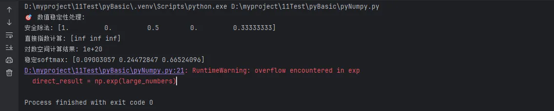
def numerical_stability_tips():
"""数值稳定性技巧"""
print("🎯 数值稳定性处理:")
# 1. 避免除零错误
denominator = np.array([1, 0, 2, 0, 3])
safe_division = np.divide(1, denominator,
out=np.zeros_like(denominator, dtype=float),
where=(denominator != 0))
print(f"安全除法: {safe_division}")
# 2. 对数空间运算
large_numbers = np.array([1e10, 1e15, 1e20])
# 直接计算可能溢出
try:
direct_result = np.exp(large_numbers)
print(f"直接指数计算: {direct_result}")
except:
print("直接计算溢出!")
# 使用log-sum-exp技巧
def log_sum_exp(x):
max_x = np.max(x)
return max_x + np.log(np.sum(np.exp(x - max_x)))
log_result = log_sum_exp(large_numbers)
print(f"对数空间计算结果: {log_result}")
# 3. 梯度下降中的数值稳定
def stable_softmax(x):
"""数值稳定的softmax函数"""
exp_x = np.exp(x - np.max(x, axis=-1, keepdims=True))
return exp_x / np.sum(exp_x, axis=-1, keepdims=True)
logits = np.array([1000, 1001, 1002]) # 很大的数值
stable_probs = stable_softmax(logits)
print(f"稳定softmax: {stable_probs}")
numerical_stability_tips()
📊 广播机制的巧妙运用
Pythondef broadcasting_examples():
"""广播机制应用示例"""
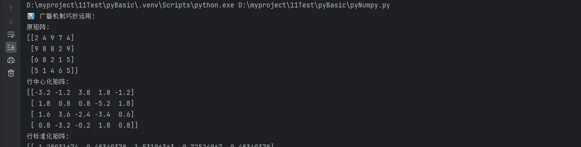
print("📊 广播机制巧妙运用:")
# 矩阵每行减去该行的平均值
matrix = np.random.randint(1, 10, (4, 5))
print(f"原矩阵:\n{matrix}")
row_means = np.mean(matrix, axis=1, keepdims=True)
centered_matrix = matrix - row_means
print(f"行中心化矩阵:\n{centered_matrix}")
# 矩阵标准化
matrix_std = (matrix - np.mean(matrix, axis=1, keepdims=True)) / np.std(matrix, axis=1, keepdims=True)
print(f"行标准化矩阵:\n{matrix_std}")
# 距离矩阵计算
points = np.random.rand(5, 2) # 5个2D点
# 使用广播计算所有点对之间的距离
distances = np.sqrt(np.sum((points[:, None, :] - points[None, :, :]) ** 2, axis=2))
print(f"距离矩阵形状: {distances.shape}")
print(f"最大距离: {np.max(distances):.4f}")
broadcasting_examples()
🚨 常见陷阱与解决方案
⚠️ 数据类型陷阱
Pythonimport time
import numpy as np
def data_type_pitfalls():
"""数据类型常见陷阱"""
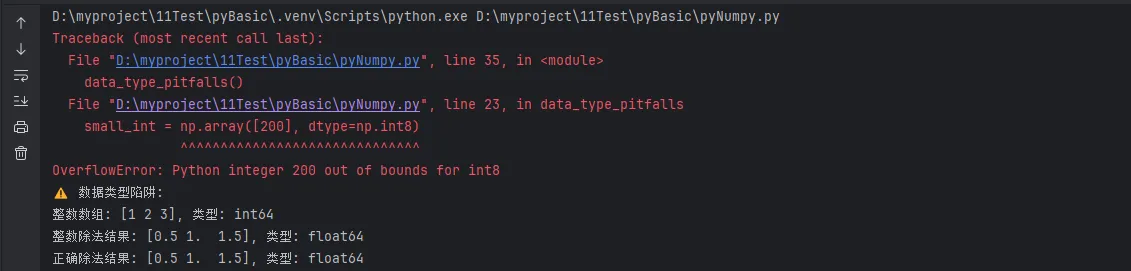
print("⚠️ 数据类型陷阱:")
# 陷阱1:整数除法
int_array = np.array([1, 2, 3], dtype=int)
print(f"整数数组: {int_array}, 类型: {int_array.dtype}")
# 错误方式
wrong_result = int_array / 2
print(f"整数除法结果: {wrong_result}, 类型: {wrong_result.dtype}")
# 正确方式
correct_result = int_array.astype(float) / 2
print(f"正确除法结果: {correct_result}, 类型: {correct_result.dtype}")
# 陷阱2:溢出问题
small_int = np.array([200], dtype=np.int8)
print(f"int8最大值: {np.iinfo(np.int8).max}")
# 溢出演示
overflow_result = small_int + 100
print(f"溢出结果: {overflow_result}") # 会回环
# 安全处理
safe_result = small_int.astype(np.int16) + 100
print(f"安全结果: {safe_result}")
data_type_pitfalls()
🔄 内存管理优化
Pythonimport time
import numpy as np
def memory_optimization():
"""内存优化技巧"""
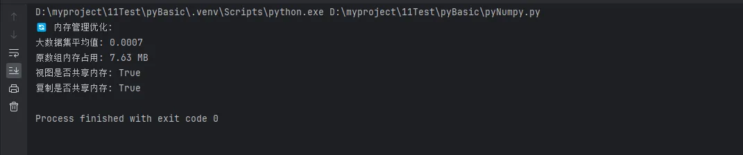
print("🔄 内存管理优化:")
# 使用生成器处理大数据
def process_large_data_generator(size=1000000):
"""生成器方式处理大数据"""
chunk_size = 10000
for i in range(0, size, chunk_size):
chunk = np.random.randn(min(chunk_size, size - i))
yield np.mean(chunk), np.std(chunk)
# 累积统计而不存储所有数据
means, stds = [], []
for mean, std in process_large_data_generator():
means.append(mean)
stds.append(std)
overall_mean = np.mean(means)
print(f"大数据集平均值: {overall_mean:.4f}")
# 视图vs复制
original = np.arange(1000000)
view = original[::2] # 视图,不占用额外内存
copy = original[::2].copy() # 复制,占用新内存
print(f"原数组内存占用: {original.nbytes / 1024 / 1024:.2f} MB")
print(f"视图是否共享内存: {view.base is original}")
print(f"复制是否共享内存: {copy.base is None}")
memory_optimization()
🎯 总结核心要点
通过本文的深入探讨,我们掌握了NumPy数学函数在Python开发中的核心应用技巧。让我们回顾三个关键要点:
🚀 性能优化是关键:NumPy的向量化运算相比原生Python能带来数十倍的性能提升,特别是在处理大规模数据时。合理使用广播机制、就地运算和批量处理,能够显著优化内存使用和计算效率。
🔧 数值稳定性不容忽视:在实际的编程技巧应用中,处理数值稳定性问题至关重要。通过合理的数据类型选择、溢出检测和对数空间运算,可以避免常见的数值计算陷阱。
💡 场景化应用最实用:无论是图像处理、金融分析还是科学计算,NumPy数学函数都提供了强大的工具支持。掌握这些实际应用场景中的最佳实践,将让你的上位机开发和数据处理工作事半功倍。
希望这篇文章能够成为你Python数值计算路上的得力助手。记住,编程技巧的掌握需要在实践中不断磨练,建议你将文中的代码示例运行一遍,并尝试应用到自己的项目中。
本文作者:技术老小子
本文链接:
版权声明:本博客所有文章除特别声明外,均采用 BY-NC-SA 许可协议。转载请注明出处!