在Python数据分析和上位机开发中，统计计算是绕不开的核心环节。无论是处理传感器数据、分析生产指标，还是进行质量控制，统计函数都扮演着关键角色。NumPy作为Python科学计算的基石，提供了丰富而高效的统计函数库。本文将从实战角度深入解析NumPy统计函数的核心功能，帮助开发者在实际项目中游刃有余地处理各类统计需求。

🎯 问题分析：为什么需要掌握NumPy统计函数？

在实际的Python开发工作中，我们经常遇到这些场景：

🔸 数据质量监控

• 需要快速计算大批量数据的均值、方差，判断数据稳定性
• 要找出异常值，进行数据清洗

🔸 生产过程控制

• 实时统计设备运行参数的分布情况
• 计算产品质量指标的置信区间

🔸 性能分析优化

• 分析算法执行时间的统计特征
• 评估系统负载的波动范围

传统的Python内置统计方法在处理大数据时性能不足，而NumPy的向量化计算能够显著提升效率，这就是我们选择NumPy统计函数的核心原因。

💡 解决方案：NumPy统计函数体系

🚀 基础描述统计

NumPy提供了完整的描述统计函数族，让我们从最常用的开始：

Python
import numpy as np

# 创建示例数据集
data = np.array([23, 45, 56, 78, 32, 67, 89, 12, 34, 56, 78, 90, 43, 21, 65])
print(f"原始数据: {data}")

# 基础统计量
print(f"均值: {np.mean(data):.2f}")
print(f"中位数: {np.median(data):.2f}")
print(f"标准差: {np.std(data):.2f}")
print(f"方差: {np.var(data):.2f}")

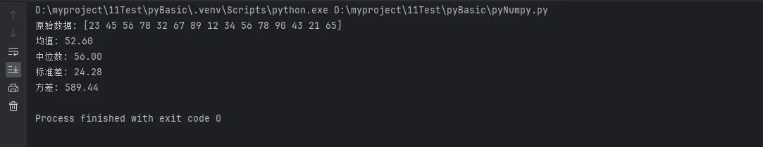
💪 实战技巧：在处理传感器数据时，通常先计算这四个基础统计量来快速了解数据分布特征。

📊 分位数与极值统计

Python
import numpy as np

# 创建示例数据集
data = np.array([23, 45, 56, 78, 32, 67, 89, 12, 34, 56, 78, 90, 43, 21, 65])
# 分位数计算
percentiles = [25, 50, 75, 90, 95]
print("分位数分析:")
for p in percentiles:
    value = np.percentile(data, p)
    print(f"  {p}%分位数: {value:.2f}")

# 极值统计
print(f"\n极值分析:")
print(f"最小值: {np.min(data)}")
print(f"最大值: {np.max(data)}")
print(f"范围: {np.ptp(data)}")  # peak to peak
print(f"最小值索引: {np.argmin(data)}")
print(f"最大值索引: {np.argmax(data)}")

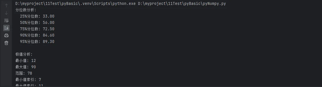
🎯 应用场景：在质量控制中，95%分位数常用于设定报警阈值，而极值统计帮助识别异常数据点。

📈 多维数组统计

NumPy的强大之处在于处理多维数组的统计计算：

Python
# 创建二维数据矩阵（模拟多传感器数据）
sensor_data = np.random.normal(50, 10, (100, 5))  # 100个时间点，5个传感器
print(f"数据形状: {sensor_data.shape}")

# 按轴统计
print("各传感器统计（按列）:")
print(f"均值: {np.mean(sensor_data, axis=0)}")
print(f"标准差: {np.std(sensor_data, axis=0)}")

print("\n各时间点统计（按行）:")
time_means = np.mean(sensor_data, axis=1)
print(f"前10个时间点均值: {time_means[:10]}")

# 全局统计
print(f"\n整体统计:")
print(f"全局均值: {np.mean(sensor_data):.2f}")
print(f"全局标准差: {np.std(sensor_data):.2f}")

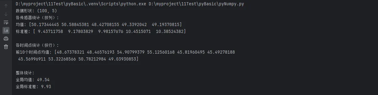
⚡ 性能优势：使用axis参数进行向量化计算，比循环方式快10-100倍。

🔥 代码实战：构建实用统计工具

📋 数据质量评估器

让我们构建一个实用的数据质量评估工具：

Python
class DataQualityAnalyzer:
    """数据质量分析器"""
    
    def __init__(self, data):
        self.data = np.array(data)
        self.stats = {}
        self._calculate_stats()
    
    def _calculate_stats(self):
        """计算基础统计指标"""
        self.stats = {
            'count': len(self.data),
            'mean': np.mean(self.data),
            'median': np.median(self.data),
            'std': np.std(self.data),
            'var': np.var(self.data),
            'min': np.min(self.data),
            'max': np.max(self.data),
            'range': np.ptp(self.data),
            'q25': np.percentile(self.data, 25),
            'q75': np.percentile(self.data, 75),
            'iqr': np.percentile(self.data, 75) - np.percentile(self.data, 25)
        }
    
    def detect_outliers(self, method='iqr'):
        """异常值检测"""
        if method == 'iqr':
            q25, q75 = self.stats['q25'], self.stats['q75']
            iqr = self.stats['iqr']
            lower_bound = q25 - 1.5 * iqr
            upper_bound = q75 + 1.5 * iqr
            
            outliers_mask = (self.data < lower_bound) | (self.data > upper_bound)
            return self.data[outliers_mask], np.where(outliers_mask)[0]
        
        elif method == 'zscore':
            z_scores = np.abs((self.data - self.stats['mean']) / self.stats['std'])
            outliers_mask = z_scores > 3
            return self.data[outliers_mask], np.where(outliers_mask)[0]
    
    def quality_report(self):
        """生成质量报告"""
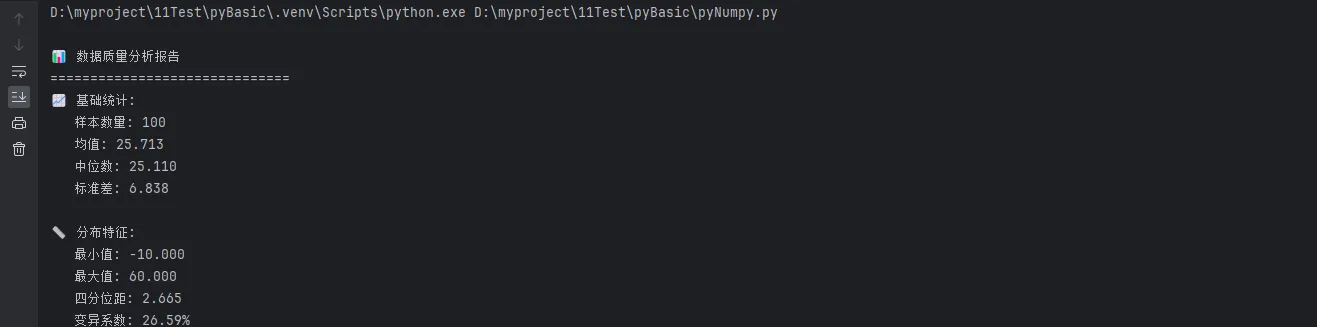
        report = f"""
📊 数据质量分析报告
{'='*30}
📈 基础统计:
   样本数量: {self.stats['count']}
   均值: {self.stats['mean']:.3f}
   中位数: {self.stats['median']:.3f}
   标准差: {self.stats['std']:.3f}
   
📏 分布特征:
   最小值: {self.stats['min']:.3f}
   最大值: {self.stats['max']:.3f}
   四分位距: {self.stats['iqr']:.3f}
   变异系数: {(self.stats['std']/self.stats['mean'])*100:.2f}%

🔍 异常检测:"""
        
        # IQR异常检测
        iqr_outliers, iqr_indices = self.detect_outliers('iqr')
        report += f"\n   IQR方法: {len(iqr_outliers)} 个异常值"
        
        # Z-score异常检测
        z_outliers, z_indices = self.detect_outliers('zscore')
        report += f"\n   Z-score方法: {len(z_outliers)} 个异常值"
        
        return report

# 实战演示
# 模拟传感器数据（包含一些异常值）
sensor_readings = np.concatenate([
    np.random.normal(25, 2, 95),  # 正常读数
    np.array([45, 50, -10, 60, 55])  # 异常值
])

analyzer = DataQualityAnalyzer(sensor_readings)
print(analyzer.quality_report())

🎯 滑动窗口统计

在实时数据处理中，滑动窗口统计非常实用：

Python
def rolling_statistics(data, window_size):
    """计算滑动窗口统计"""
    data = np.array(data)
    n = len(data)
    
    if window_size > n:
        raise ValueError("窗口大小不能大于数据长度")
    
    # 预分配结果数组
    result_length = n - window_size + 1
    means = np.zeros(result_length)
    stds = np.zeros(result_length)
    
    # 向量化计算滑动统计
    for i in range(result_length):
        window = data[i:i+window_size]
        means[i] = np.mean(window)
        stds[i] = np.std(window)
    
    return means, stds

# 更高效的实现方式
def fast_rolling_mean(data, window_size):
    """快速滑动均值计算"""
    data = np.array(data)
    
    # 使用卷积实现高效滑动计算
    kernel = np.ones(window_size) / window_size
    return np.convolve(data, kernel, mode='valid')

# 实战测试
test_data = np.random.normal(100, 15, 1000)
window = 20

# 传统方法
means1, stds1 = rolling_statistics(test_data, window)

# 优化方法
means2 = fast_rolling_mean(test_data, window)

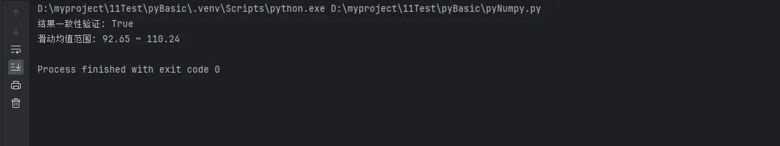
print(f"结果一致性验证: {np.allclose(means1, means2)}")
print(f"滑动均值范围: {np.min(means2):.2f} ~ {np.max(means2):.2f}")

📊 相关性分析工具

Python
def correlation_analysis(data_matrix, labels=None):
    """多变量相关性分析"""
    data = np.array(data_matrix)
    
    # 计算相关系数矩阵
    corr_matrix = np.corrcoef(data.T)  # 转置以按列计算
    
    # 生成分析报告
    n_vars = corr_matrix.shape[0]
    
    if labels is None:
        labels = [f"变量{i+1}" for i in range(n_vars)]
    
    print("🔗 变量相关性分析")
    print("="*40)
    
    # 强相关性识别（|r| > 0.7）
    strong_correlations = []
    for i in range(n_vars):
        for j in range(i+1, n_vars):
            corr_val = corr_matrix[i, j]
            if abs(corr_val) > 0.7:
                strong_correlations.append((labels[i], labels[j], corr_val))
    
    if strong_correlations:
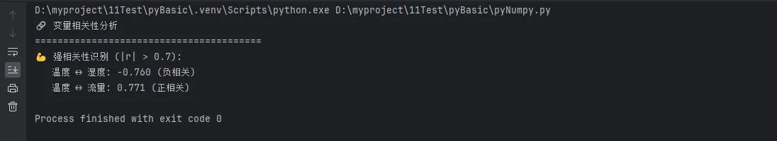
        print("💪 强相关性识别 (|r| > 0.7):")
        for var1, var2, corr in strong_correlations:
            direction = "正" if corr > 0 else "负"
            print(f"   {var1} ↔ {var2}: {corr:.3f} ({direction}相关)")
    else:
        print("   未发现强相关性")
    
    return corr_matrix

# 实战演示
# 模拟多传感器数据（温度、湿度、压力、流量）
np.random.seed(42)
temperature = np.random.normal(25, 5, 200)
humidity = 80 - 0.8 * temperature + np.random.normal(0, 3, 200)  # 与温度负相关
pressure = np.random.normal(1013, 10, 200)
flow_rate = 0.5 * temperature + np.random.normal(0, 2, 200)  # 与温度正相关

sensor_matrix = np.column_stack([temperature, humidity, pressure, flow_rate])
sensor_labels = ['温度', '湿度', '气压', '流量']

corr_result = correlation_analysis(sensor_matrix, sensor_labels)

⚡ 性能优化技巧

🚄 内存高效的大数据统计

Python
def efficient_large_data_stats(data_generator, chunk_size=10000):
    """内存友好的大数据统计计算"""
    count = 0
    sum_x = 0
    sum_x2 = 0
    min_val = float('inf')
    max_val = float('-inf')
    
    # 分块处理
    for chunk in data_generator:
        chunk = np.array(chunk)
        
        count += len(chunk)
        sum_x += np.sum(chunk)
        sum_x2 += np.sum(chunk**2)
        min_val = min(min_val, np.min(chunk))
        max_val = max(max_val, np.max(chunk))
    
    # 计算统计量
    mean = sum_x / count
    variance = (sum_x2 - sum_x**2/count) / (count - 1)
    std = np.sqrt(variance)
    
    return {
        'count': count,
        'mean': mean,
        'std': std,
        'min': min_val,
        'max': max_val,
        'range': max_val - min_val
    }

# 模拟大数据流
def data_stream_generator(total_size=1000000, chunk_size=10000):
    """数据流生成器"""
    for i in range(0, total_size, chunk_size):
        chunk_end = min(i + chunk_size, total_size)
        yield np.random.normal(50, 10, chunk_end - i)

# 测试大数据统计
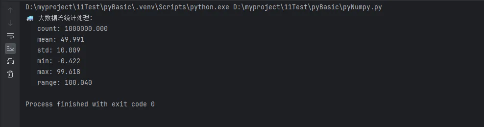
print("🚄 大数据流统计处理:")
large_stats = efficient_large_data_stats(data_stream_generator())
for key, value in large_stats.items():
    print(f"   {key}: {value:.3f}")

🎯 向量化vs循环性能对比

Python
import time

def performance_comparison():
    """性能对比测试"""
    # 生成测试数据
    data = np.random.normal(0, 1, (1000, 1000))
    
    # 方法1: 向量化计算
    start_time = time.time()
    vectorized_mean = np.mean(data, axis=1)
    vectorized_std = np.std(data, axis=1)
    vectorized_time = time.time() - start_time
    
    # 方法2: 循环计算
    start_time = time.time()
    loop_means = []
    loop_stds = []
    for row in data:
        loop_means.append(np.mean(row))
        loop_stds.append(np.std(row))
    loop_time = time.time() - start_time
    
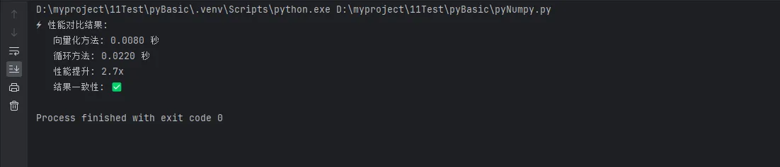
    print("⚡ 性能对比结果:")
    print(f"   向量化方法: {vectorized_time:.4f} 秒")
    print(f"   循环方法: {loop_time:.4f} 秒")
    print(f"   性能提升: {loop_time/vectorized_time:.1f}x")
    
    # 验证结果一致性
    results_match = np.allclose(vectorized_mean, loop_means)
    print(f"   结果一致性: {'✅' if results_match else '❌'}")

performance_comparison()

🎯 总结与实战要点

通过本文的深入解析，我们掌握了NumPy统计函数的核心应用技能。三个关键要点需要牢记：

🚀 性能优先：始终选择向量化计算而非循环，利用axis参数进行多维统计，在大数据场景下采用分块处理策略。

💡 实用至上：构建可复用的统计分析工具类，结合异常检测、滑动窗口等实战技巧，让代码直接服务于项目需求。

🔧 优化思维：深入理解NumPy的内存管理机制，合理选择统计方法，在准确性和效率之间找到最佳平衡点。

NumPy统计函数不仅是数据分析的利器，更是Python开发者提升编程技巧的重要工具。掌握这些核心技能，让你在面对复杂的数据处理任务时游刃有余，在上位机开发和系统优化中展现专业实力。持续实践这些技巧，你将发现数据分析变得如此高效而优雅！